Running an Analysis: General steps and ORA

We suggest that you read this page first, as it explains some aspects of analysis that are common to all the methods.

Overview of enrichment analysis

ErmineJ provides a range of methods for performing “enrichment analysis”. What is that? The most common analogy used to explain the basic idea is the Urn problem. An analogy more relevant to 21st century humans is the iPod shuffle problem. If your music player seems to be serving up too much Chopin or Lady Gaga, you might question whether it is really random. The idea of “more Chopin than I expected” is intuitive, but humans are bad at figuring out the probabilities. In science, such misjudgements can have more serious consequences, so we use statistical techniques to tell us how surprised we should be.

For genomics applications, we think of genes as items that can be “chosen” by you, typically using a laboratory experiment. We want to know if the experiment is picking genes randomly with respect to some criteria. The criteria of typical interest is something akin to “genes in a pathway” or “function”, though other criteria can be used (such as “genes on a chromosome”, or even something silly like “genes with names that start with the letter ‘M'”).

To make it a bit more concrete, assuming for the moment you have a list of 100 genes that were “chosen” by your experiment, we might want to know: “There are 12 genes involved in the cell cycle in my 100 genes. Is that surprising?”

The answer to this question depends on how many cell cycle genes there are in total among the genes that the 100 were selected from. Thus if the genome in question has 10,000 genes, and there are 1000 cell cycle genes, by chance we’d expect about 100*1000/10,000 = 10 cell cycle genes when we pick 100 genes. Thus getting 12 is probably slightly surprising (12 > 10). The exact probabilities can be computed (subject to some important assumptions).

If this is still obscure, the iPod analogy might help. Say you have one Lady Gaga album of 10 songs, out of 1000 songs on your music player. This means that if the shuffle mode is random, each time you listen to a song, there is a 10/1000 = 1% chance of it being by Lady Gaga, assuming repeats are allowed. Now say today you listened to 30 songs on “shuffle”, of which 4 happen to be by Lady Gaga. That’s over 13%, which is a lot more than we’d expect. We would have good reason to be suspicious about the randomness of our music player.

ErmineJ was actually designed to deal with a slightly more complex situation: We don’t have 100 genes selected out of 10,000, but we do have a ranking of the 10,000 genes (possibly with a score). The most common way to get such a ranking is from an analysis that looks at each gene and assigns a p-value. A typical example would be a differential expression analysis. But the basic idea is the same: we want to know if the cell cycle genes are “surprisingly near the top of the ranking”.

Naturally we might not know ahead of time that we want to look at the “cell cycle”; thus it is usual to use a set of gene groups (“functions”, “chromosomes”, whatever). A common source of these groupings is the Gene Ontology, but there is no limit to how they could be created (including the silly example of the first letter of the English gene name, which would yield 26 groups to test).

Thus ErmineJ is appropriate to use if you have a list of genes. How you generate this list is up to you; ErmineJ tries to be flexible. It can be a list of “hits” (like the 100 genes in the example) or a set of scores for all the genes that can be ranked.

To summarize, you can do an enrichment analysis if you have the following:

A list of genes you want to analyze. These are unique to your analysis.
A reference set of gene groups that you want to test for enrichment in your list. These are often provided by someone else.

Note that ErmineJ offers an additional method that doesn’t use gene scores, the correlation method.

Overview of the ORA method

Over-representation analysis (ORA) examines the genes that meet a selection criterion and determines if there are gene sets which are statistically over-represented in that list. This method differs from other methods provided by ErmineJ in that you must set a gene score threshold for gene selection, or define a “hit list” of genes.

Technical comment: The probabilities produced by ErmineJ ORA are computed using the hypergeometric distribution, but falls back to using the binomial approximation as needed.

When to use ORA

ORA is not the preferred method in ErmineJ. In fact ErmineJ was developed to help disseminate a method based on rankings of genes (Gene Score Resampling). More recently support for the “ROC” and “precision-recall” method was added.

Because ORA requires that you set a distinction between “good” and “bad” genes, ORA is most appropriate when you are very confident about the threshold. This is because changing the threshold can change the results, sometimes dramatically. If you are examining genes which naturally fall into two categories (“on chromosome 2” and “not on chromosome 2”), then ORA is the logical choice. Otherwise, in our opinion the other methods are more appropriate.

We are sometimes asked about looking at functional enrichment in gene clusters. ORA might seem like a natural choice because for each cluster you divide the genes into “in the cluster” and “not in the cluster”. ORA is appropriate in that case, but ErmineJ also offers an alternative, correlation scoring.

Walkthrough

Step 1: Choose type of analysis

Here we selected ORA:

Step 2: Choose input file(s)

The next window is common to all analysis methods. Two data files are requested. For ORA, only the Gene Score File is required. However, entering the raw data file will allow you to visualize the results later.

The Gene Score file format is explained here. In this panel, you must also select the score column. The first column in the gene score file contains the probe identifiers; the gene scores themselves are in the second or higher column. If your gene score file only has two columns, just use the default value of 2. An example (to be used with platform GPL91) is here.

The Raw data file format is explained here. An example (to be used with platform GPL91) is here.

ORA only: Quick lists

As of ErmineJ 3, you also have the option of using a “Quick list”. Paste or type in a list of gene identifiers, as shown below. ErmineJ will automatically create an appropriate temporary Gene Score file for you. You may give a name to the list, which will be used in the file name.

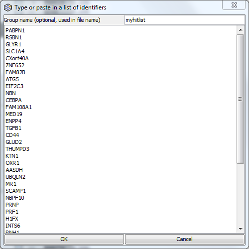
Additional things to know about Quick Lists:

Identifiers can be delimited by new lines, commas, spaces or pipe symbols (“|”), or a mixture.
Matching of identifiers is case insensitive, so ABC1 is the same as abc1, and any extra white space is ignored.
You can use identifiers from either of the first two columns of your annotation file. For example, for microarrays this would be the probe ID (first column) or gene symbol (second column). Probe IDs and gene symbols can be mixed.
The scores that are generated are set up to match your current “log transform” and “bigger is better” setting. This has implications for re-using Quick List files as noted below.
A score file will be generated and saved in your designated ermineJ data directory (e.g., $HOME/ermineJ.data), with a name like QuickList.1949490.txt

Note that using a Quick List has the following effects on your settings.

The score column will be set to 2.
The score threshold will be set to 1.0 (or, if you have log transformation disabled, it will be set to 0.0)
The file created holding your quick list scores becomes your default score file (that is, it is listed in your ermineJ.properties file).

Be careful if you re-use Quick List files. If you change the “score threshold”, “score column”, “bigger is better” and “log transform” settings, the quick list score file might not be appropriate. Future uses of the files require the same attention to settings as the use of any other user-provided gene score file.

Step 3: Choose GO aspect or custom gene sets to include

Step 3 is also common to all the methods. Select the GO aspects you want to include in the analysis.

Step 4: Choose class size range and how repeated genes are handled

Step 4 is also common to all the methods.

The maximum and minimum gene set sizes determine the range of gene set sizes that will be considered. We recommend avoiding the use of very small or very large gene sets. There are several reasons to avoid using extremes:

The more gene sets you examine, the worse the multiple testing issue.
Using more gene sets increases computation time for the resamping-based methods (not an issue for ORA).
Very large or very small gene sets are less informative:
- Very large gene sets are rather non-specific and tend not to tell you as much.
- Very small gene sets defeat the purpose of examining genes in groups.

The ” Gene replicate treatment ” refers to what is done when a gene occurs more than once in the dataset.

There are two options, “Best” and “Mean”. The application of these methods differs for the different methods. There is more information here

Step 5: ORA-specific settings

This step is specific to the ORA analysis. Equivalent

Important: if you are using a Quick List, you should probably not change these settings, as the Quick List score file is generated based on your last used settings.

Gene score threshold

The gene score threshold determines how genes are “selected”. Genes that meet the threshold requirement are considered “good”. ErmineJ operates differently from some other available tools in that you do not enter the “good” genes yourself: the software selects them based on the criteria you set here.

The value you set here refers to the value in your original scores. Thus if you have p-values, your threshold might be 0.0001, not 4.0, even if you check “log transform” (see below).

After you change this setting, the number of genes selected and their multifunctionality bias are displayed in the status bar of the wizard. This value is also reported in the tooltip for the results header (after the analysis). Multifunctionality bias is the tendency for your selected genes to contain genes with many functions. The value provided is the area under the ROC curve (AUROC). Values of 0.5 are uninteresting, while values nearer to 1.0 would indicate some degree of multifunctionality bias.

Tip: If you are using raw p values as your gene scores, make sure your threshold is a value between 0 and 1 (e.g., 0.0001), check the “log transform” box, and leave the “larger scores are better” box unchecked. This is because the “larger is better” choice relates to the original threshold, not the log-transformed threshold. On the other hand, if your p-values are already -log-transformed, you should use the exact opposite settings.

Log transformation

If you negative log-transform the gene scores, then your input gene scores are transformed according to the function f(x) = – log₁₀ (x). If you are using p-values as your input, you should check this box but leave the “larger scores are better” box unchecked, as this refers to your original scores (and smaller p-values are better).

If your input is already -log transformed, then you uncheck the log-transformation box and check the “larger scores are better” box.

Are larger gene scores better?

If you are using fold change as your gene scores, you will probably want to check the “larger scores are better” box. This assumes that you have taken the absolute value of the fold change values before entering them into ermineJ. That way, changes up and down will be considered equally. Alternatively, you could focus on changes up or down by retaining the sign on the fold change values and setting this option depending on which direction of change you are interested in analyzing.

There is another explanation of gene scores here.

Multifunctionality correction

As described here, the presence of highly multifunctional genes in your “hit list” can strongly distort the results of over-representation analysis. There is no drawback to checking the box, except computation takes a little longer.

Run the analysis

After clicking “finish”, you will rapidly get a new result set in the output (results) table. This is explained here.